
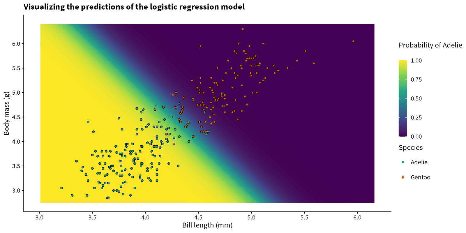
Despite its misleading name, Logistic Regression is not a regression algorithm used to predict continuous numbers like prices or temperatures. Instead, it is one of the most fundamental and widely used algorithms for binary classification—predicting which of two discrete categories an observation belongs to.
Whether your model needs to classify emails as
Spam or Not Spam, evaluate whether a transaction is Fraudulent or Legitimate, or predict if a patient has a specific medical condition, logistic regression is often the go-to baseline algorithm.Here is a simple, intuitive breakdown of how logistic regression works under the hood.
The Core Concept: From Linear to Logistic
To understand logistic regression, it helps to start with Linear Regression.
Linear regression predicts continuous numerical outcomes by fitting a straight line equation to the data:
$$y = mX + b$$
However, using a straight line for classification creates a major problem: a linear equation outputs values from $-\infty$ to $+\infty$. Probabilities, by definition, must strictly fall between $0.0$ ($0\%$) and $1.0$ ($100\%$).
Linear Output (-∞ to +∞) ──► [ Sigmoid Function ] ──► Probability Output (0.0 to 1.0)
Logistic regression solves this by taking the linear equation and passing its raw output through a special mathematical S-shaped curve called the Sigmoid Function (or Logistic Function).
The Math Made Simple: The Sigmoid Function
The Sigmoid Function squashes any real-numbered input into an output value strictly bounded between $0$ and $1$, representing a valid probability:
$$\sigma(z) = \frac{1}{1 + e^{-z}}$$
Where:
-
$z = \beta_0 + \beta_1 X_1 + \beta_2 X_2 + \dots + \beta_n X_n$ (the weighted sum of input features).
-
$e$ is Euler’s constant ($\approx 2.718$).
                        The Sigmoid Curve
             1.0 ┼───────────────────────╭──────
                 │                      ┆
                 │                     ╭┘
                 │                    ╭┘
             0.5 ┼───────────────────┼──────────  Threshold Cutoff
                 │                 ╭┘
                 │                ╭┘
                 │  ──────╯      ┆
             0.0 ┼───────────────────────┴──────
                -6    -4    -2   0   2   4   6
                                 z
How the Sigmoid Interprets Values:
-
If $z$ is a large positive number, $\sigma(z)$ approaches $1.0$.
-
If $z$ is a large negative number, $\sigma(z)$ approaches $0.0$.
-
If $z = 0$, $\sigma(z) = \mathbf{0.5}$ exactly.
Decision Boundaries & Odds Ratios
1. The Decision Boundary
Once the sigmoid function outputs a probability value (e.g., $P(Y=1 \vert{} X) = 0.78$), the algorithm applies a threshold cutoff (default is usually $0.5$) to make a final categorical decision:
$$\text{Predicted Class} = \begin{cases} 1 (\text{Positive}) & \text{if } P(Y=1) \ge 0.5 \\ 0 (\text{Negative}) & \text{if } P(Y=1) < 0.5 \end{cases}$$
The point where the model switches its prediction from Class $0$ to Class $1$ is called the Decision Boundary.
2. Odds Ratios and Log-Odds
Logistic regression models the logarithm of the odds (log-odds) of the positive outcome occurring:
$$\ln\left(\frac{P}{1 – P}\right) = \beta_0 + \beta_1 X_1$$
Where $\frac{P}{1-P}$ represents the Odds Ratio. This linear relationship between independent variables and the log-odds makes logistic regression highly interpretable compared to black-box models.
How Logistic Regression Learns: Loss Function
Linear regression uses Mean Squared Error (MSE) to minimize errors. However, applying MSE to a non-linear sigmoid curve results in a non-convex function full of local minima, making optimization unreliable.
Instead, logistic regression uses Binary Cross-Entropy Loss (also known as Log Loss):
$$\text{Cost}(y, \hat{y}) = – \left[ y \log(\hat{y}) + (1 – y) \log(1 – \hat{y}) \right]$$
Where:
-
$y$ is the actual label ($0$ or $1$).
-
$\hat{y}$ is the predicted probability.
Why Log Loss Works:
-
If the true label is $1$ and the model predicts $0.99$, the penalty/loss is near $0$.
-
If the true label is $1$ and the model predicts $0.01$, the penalty/loss approaches infinity. This heavily penalizes confident wrong predictions during gradient descent updates.
Strengths vs. Limitations
| Advantages | Limitations |
| Highly Interpretable: Coefficients show feature direction & strength | Assumes linear decision boundaries between features |
| Probability Outputs: Provides confidence scores, not just rigid labels | Struggles with complex, non-linear relationships without feature engineering |
| Computationally Light: Fast to train and predict in production | Sensitive to severe outliers and high multicollinearity |
| Low Overfitting Risk: Less prone to overfitting on smaller datasets | Performs poorly when classes are heavily overlapped |
Practical Python Implementation
Building a logistic regression classifier in Python using
scikit-learn takes only a few lines:Python
from sklearn.model_selection import train_test_split
from sklearn.linear_model import LogisticRegression
from sklearn.metrics import classification_report

# 1. Split training and testing sets
X_train, X_test, y_train, y_test = train_test_split(X, y, test_size=0.2, random_state=42)

# 2. Instantiate and fit model
model = LogisticRegression()
model.fit(X_train, y_train)

# 3. Get predicted class labels and probabilities
y_pred = model.predict(X_test)
y_probs = model.predict_proba(X_test)[:, 1] # Probability of Class 1

# 4. Print performance metrics
print(classification_report(y_test, y_pred))
Key Takeaway
Logistic Regression is essentially linear regression wrapped inside a sigmoid curve. It translates linear combinations of input features into clean $0$-to-$1$ probabilities, making it the industry-standard starting point for binary classification tasks.