
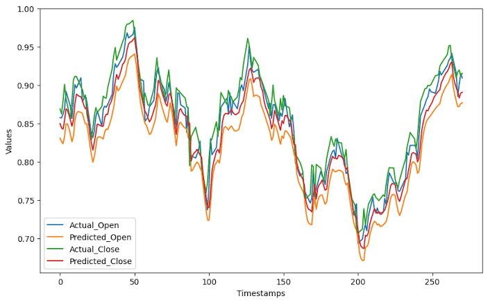
From anticipating inventory demand in retail supply chains to predicting financial market fluctuations, electricity grid loads, and web traffic spikes, Time Series Forecasting is one of the most widely applied disciplines in data science.
Unlike standard tabular datasets where observations are assumed to be independent and identically distributed (i.i.d.), time series data exhibits inherent chronological dependencies. The sequence and timing of data points carry critical predictive signals that require specialized modeling techniques.
Here is a practical guide to understanding time series components, core forecasting methodologies, and best evaluation practices.
1. Anatomy of Time Series Data
Before applying forecasting models, a time series must be decomposed into its underlying constituent components:
Original Series = Trend Component + Seasonal Component + Residual (Noise)
Core Components
-
Trend ($T_t$): The long-term directional movement in the data (increasing, decreasing, or stationary over prolonged periods).
-
Seasonality ($S_t$): Fixed, repeating cyclic patterns that occur at regular intervals (e.g., daily surges in traffic, annual holiday sales spikes).
-
Cyclical ($C_t$): Fluctuation patterns that repeat without fixed frequencies (e.g., multi-year economic boom-and-bust cycles).
-
Irregular/Noise ($I_t$): Unpredictable random variance or residual noise remaining after removing systematic signals.
Stationarity
A time series is stationary if its statistical properties—such as mean, variance, and autocorrelation—remain constant over time. Most classical statistical models require non-stationary series to be transformed into stationary ones (via differencing or log transformations) before modeling.
2. Classical Statistical Methods
Classical statistical approaches excel on univariate data with clear parametric properties and historical patterns.
                         Statistical Model Hierarchy
                                      │
           ┌──────────────────────────┴──────────────────────────┐
           ▼                                                     ▼
     [ ARIMA ]                                             [ SARIMA ]
  (Autoregressive Integrated                             (Seasonal ARIMA)
   Moving Average)                                       • Adds seasonal terms (P, D, Q)s
  • Handles non-seasonal trends                          • Captures repeating calendar cycles
A. Autoregressive (AR) Models
Predicts future values using a linear combination of past observations (lags):
$$y_t = c + \phi_1 y_{t-1} + \phi_2 y_{t-2} + \dots + \phi_p y_{t-p} + \epsilon_t$$
B. Moving Average (MA) Models
Predicts future values using past forecast errors (residuals):
$$y_t = \mu + \epsilon_t + \theta_1 \epsilon_{t-1} + \theta_2 \epsilon_{t-2} + \dots + \theta_q \epsilon_{t-q}$$
C. ARIMA($p, d, q$)
Combines Autoregression ($p$), Differencing ($d$) to achieve stationarity, and Moving Average ($q$).
-
$p$ (AR order): Number of lag observations included.
-
$d$ (Degree of Differencing): Number of times raw observations are subtracted from previous values to stabilize the mean.
-
$q$ (MA order): Size of the moving average window applied to lagged errors.
D. SARIMA($p,d,q$)($P,D,Q$)$_s$
Extends ARIMA by incorporating explicit seasonal parameters ($P, D, Q$) over a fixed seasonal period $s$ (e.g., $s=12$ for monthly data with annual seasonality).
3. Machine Learning Approaches
When dealing with complex non-linear relationships, multi-variate exogenous features, or thousands of interrelated time series, modern machine learning algorithms often outperform classical methods.
Raw Time Series Data ──► Feature Engineering (Lags, Rolling Means) ──► Gradient Boosted Trees (XGBoost)
Feature Engineering for Time Series ML
To train supervised machine learning models (like XGBoost, LightGBM, or Random Forests) on sequential data, time series must be restructured into tabular feature matrices:
-
Lag Features: $y_{t-1}, y_{t-2}, y_{t-7}$ (past values used as direct predictors).
-
Rolling Window Statistics: Moving averages, rolling standard deviations, min/max over sliding windows (e.g., 7-day mean).
-
Calendar Features: Extracting explicit categorical signals like day-of-week, month, quarter, holiday flags.
Machine Learning & Deep Learning Architectures
-
Tree Ensembles (XGBoost/LightGBM): Highly effective when augmented with lag and calendar features; naturally handles non-linearities and exogenous variables.
-
Neural Prophet / Prophet: Additive regression models developed for business forecasting featuring intuitive parameter tuning for trends, holiday impacts, and custom seasonality.
-
LSTMs & Temporal Fusion Transformers (TFT): Deep learning network architectures specifically built to capture long-range temporal dependencies across massive multi-variate datasets.
4. Model Selection Matrix
| Method | Best For | Pros | Cons |
| Simple Exponential Smoothing | Short-term trends without seasonality | Simple, fast execution, low data requirement | Cannot handle strong seasonality or long horizons |
| ARIMA / SARIMA | Univariate series with clear statistical structure | Well-established theoretical foundation, interpretable | Struggles with multi-variate exogenous features and non-linearities |
| XGBoost / LightGBM | High-dimensional data with exogenous predictors | High accuracy, scales well, captures non-linearities | Requires careful lag/rolling feature engineering |
| Prophet | Business time series with missing data & strong seasonality | Robust to outliers/missing data, easy to interpret | May underperform on complex multi-seasonal structural shifts |
5. Time Series Cross-Validation & Metrics
Standard $K$-Fold cross-validation cannot be used for time series because randomly shuffling data causes data leakage from the future into the past.
Time Series Split (Expanding Window)
Use a Rolling/Expanding Window approach that trains exclusively on historical data prior to the evaluation window:
Fold 1: [ Train: Jan-Mar ] ──► [ Test: Apr ]
Fold 2: [ Train: Jan-Apr ] ──────► [ Test: May ]
Fold 3: [ Train: Jan-May ] ──────────► [ Test: Jun ]
Specialized Evaluation Metrics
-
MAE (Mean Absolute Error): Measures average absolute deviation; easy to interpret in original units.
-
RMSE (Root Mean Squared Error): Penalizes larger forecast errors more heavily.
-
MAPE (Mean Absolute Percentage Error): Scale-independent percentage metric; fails if actual values contain zero.
-
MASE (Mean Absolute Scaled Error): Compares model error against a naive benchmark model; suitable for comparing across different scales.
Key Takeaway
Successful time series forecasting requires matching data characteristics to model capabilities. Start by analyzing stationarity, trend, and seasonality. Use classical methods like SARIMA for baseline univariate series, and transition to feature-engineered Tree Ensembles or deep architectures when incorporating complex exogenous signals.