
The ultimate goal of any supervised machine learning algorithm is to learn patterns from training data and accurately generalize those predictions to unseen, real-world data.
However, models rarely achieve perfect accuracy. When a model makes prediction errors, those errors can almost always be decomposed into two distinct mathematical components: Bias and Variance.
The challenge is that decreasing one component often increases the other. Striking the optimal balance between the two is known as the Bias-Variance Tradeoff—one of the most foundational concepts in machine learning theory and applied model tuning.
Defining Bias and Variance
To understand the tradeoff, we must first break down what each error term represents.
                  Low Variance               High Variance
            ┌──────────────────────┐   ┌──────────────────────┐
            │       🎯             │   │      🎯  •   •       │
  Low Bias  │      •••             │   │         •   •        │
            │                      │   │        •  •          │
            └──────────────────────┘   └──────────────────────┘
            ┌──────────────────────┐   ┌──────────────────────┐
            │       🎯             │   │       🎯             │
 High Bias  │        •             │   │     •     •          │
            │       ••             │   │   •         •        │
            └──────────────────────┘   └──────────────────────┘
1. What is Bias? (Error due to overly simplistic assumptions)
Bias measures how far off the average prediction of a model is from the true underlying values. High bias occurs when an algorithm makes overly simplistic assumptions about the data structure.
-
Symptom: Underfitting. The model performs poorly on both training data and testing data.
-
Example: Fitting a straight line (Linear Regression) to data that clearly follows a complex curve.
-
Characteristics: High error rate, inflexible, fails to capture complex feature relationships.
2. What is Variance? (Error due to sensitivity to training fluctuations)
Variance measures how much a model’s predictions fluctuate when trained on different random subsets of the same population dataset. High variance occurs when an algorithm learns the training data too closely, including its random noise and anomalies.
-
Symptom: Overfitting. The model performs exceptionally well on training data but poorly on testing data.
-
Example: An unconstrained Decision Tree trained until every leaf node isolates a single training instance.
-
Characteristics: Extremely flexible, memorizes training noise, highly unstable predictions on unseen data.
The Mathematical Breakdown: Total Error Formula
Mathematically, the total expected prediction error (Mean Squared Error) of a model at a given data point can be decomposed into three distinct parts:
$$\text{Total Error} = \text{Bias}^2 + \text{Variance} + \text{Irreducible Error}$$
Where:
-
$\text{Bias}^2$: Systemic error introduced by model simplification.
-
$\text{Variance}$: Variability in predictions across different training iterations.
-
$\text{Irreducible Error}$ ($\sigma^2$): Noise inherently present in the data collection process (e.g., sensor inaccuracies, missing variables). No model can eliminate irreducible error.
The Tradeoff Curve Explained
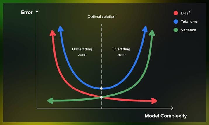
As model complexity increases (e.g., adding more parameters, higher polynomial degrees, deeper tree depths), bias decreases, but variance simultaneously increases.
  Error
    ▲
    │ \                                                 / High Variance
    │  \                                               /  (Overfitting)
    │   \  High Bias                                  /
    │    \ (Underfitting)           Total Error      /
    │     \                            ╭─╮          /
    │      \                          ╭╯ ╰╮        /
    │       \                       ╭─╯   ╰─╮     /
    │        \                     ╭╯       ╰─╮  /
    │         ╰───────────────────╯           ╰─/────────────────
    │           Optimal Model Complexity       /  Bias^2
    └─────────────────────────────────────────┴─────────────────────►
    Simple                                                   Complex
                         Model Complexity
-
Underfitted Zone (Left): Model is too simple $\rightarrow$ High Bias, Low Variance.
-
Overfitted Zone (Right): Model is too complex $\rightarrow$ Low Bias, High Variance.
-
Sweet Spot (Center): The point where Total Error reaches its global minimum, balancing both terms for maximum generalization.
Model Spectrum: Where Do Popular Algorithms Fall?
Different machine learning algorithms carry inherent tendencies toward high bias or high variance out of the box:
| High Bias / Low Variance (Simpler) | Balanced / Adaptable | High Variance / Low Bias (Complex) |
| Linear Regression | Random Forests | Unconstrained Decision Trees |
| Logistic Regression | Gradient Boosted Trees (XGBoost) | $K$-Nearest Neighbors ($K=1$) |
| Naive Bayes | Support Vector Machines (RBF Kernel) | Deep Neural Networks (unregularized) |
Practical Strategies to Fix Bias vs. Variance Issues
When auditing your model performance across training and validation splits, use these targeted remedies depending on which issue is dominating:
How to Fix High Bias (Underfitting)
-
Increase model complexity: Add non-linear features or polynomial terms ($X^2, X^3$).
-
Decrease regularization: Reduce penalties like $L_1$ (Lasso) or $L_2$ (Ridge) strength ($\alpha / \lambda$).
-
Engineer richer features: Introduce interaction terms and contextual variables.
-
Switch algorithms: Upgrade from linear models to tree-based ensembles or neural networks.
How to Fix High Variance (Overfitting)
-
Gather more training data: More samples dilute the impact of local noise.
-
Reduce feature dimension: Apply feature selection or Principal Component Analysis (PCA).
-
Apply regularization: Enforce penalties on coefficient magnitudes ($L_1/L_2$ regularization) or add Dropout layers in deep learning.
-
Use Ensemble Bagging: Combine predictions across multiple independent models (e.g., Random Forests).
-
Early Stopping: Terminate training iterations before the validation error begins climbing.
Key Takeaway
Building high-performing machine learning models is fundamentally an exercise in managing the bias-variance tradeoff. Aim for a model complex enough to capture underlying structural signals (low bias), but constrained enough that it does not memorize random noise (low variance).