
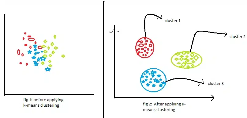
K-Means Clustering is one of the most popular, intuitive, and widely deployed unsupervised machine learning algorithms. Unlike supervised learning algorithms that rely on explicit ground-truth labels, K-Means explores unlabeled data to discover natural groupings or patterns automatically.
Whether you are segmenting e-commerce customers by purchase behavior, compressing digital images, or grouping documents by topic, K-Means provides a computationally efficient way to uncover hidden structure in high-dimensional data.
Here is a complete guide to understanding how K-Means works, how to tune its parameters, and when to apply it in production.
What is K-Means Clustering?
K-Means is a centroid-based, partition-based clustering algorithm. Its objective is simple: partition a dataset of $N$ observations into $K$ distinct, non-overlapping subgroups (clusters), where every observation belongs to the cluster with the nearest mean (centroid).
Unlabeled Data Points ──► Assign to Nearest Centroid ──► Update Centroids ──► Converged Clusters
The algorithm minimizes the within-cluster sum of squares (WCSS)—also referred to as inertia:
$$\text{WCSS} = \sum_{k=1}^{K} \sum_{x_i \in C_k} \Vert{} x_i – \mu_k \Vert{}^2$$
Where:
-
$K$ is the total number of clusters.
-
$C_k$ is the set of data points belonging to cluster $k$.
-
$x_i$ is an individual data point.
-
$\mu_k$ is the centroid (mean vector) of cluster $k$.
-
$\Vert{} x_i – \mu_k \Vert{}$ represents the Euclidean distance between point $x_i$ and centroid $\mu_k$.
How K-Means Works: Step-by-Step
K-Means uses an iterative optimization algorithm known as Expectation-Maximization (EM) to reach convergence.
┌───────────────────────────┐
│ 1. Choose K & Init Means  │
└─────────────┬─────────────┘
              │
              ▼
┌───────────────────────────┐
│ 2. Assign Points to       │ ◄─────────────────┐
│    Nearest Centroid       │                   │
└─────────────┬─────────────┘                   │ Iteration Loop
              │                                 │ (Until Convergence)
              ▼                                 │
┌───────────────────────────┐                   │
│ 3. Recalculate Centroids  │ ──────────────────┘
│    (Mean of assigned pts) │
└─────────────┬─────────────┘
              │ (No centroid movement)
              ▼
┌───────────────────────────┐
│   4. Convergence Reached  │
└───────────────────────────┘
Step 1: Initialize $K$ Centroids
Select $K$ initial points to serve as cluster centers. Standard K-Means picks $K$ random data points, while modern implementations default to K-Means++—a smart initialization strategy that spreads initial centroids far apart to accelerate convergence and avoid poor local minima.
Step 2: Assign Data Points (Expectation Step)
Calculate the Euclidean distance between each data point $x_i$ and all $K$ centroids. Assign each data point to its closest centroid:
$$d(x_i, \mu_k) = \sqrt{\sum_{j=1}^{m} (x_{ij} – \mu_{kj})^2}$$
Step 3: Update Centroids (Maximization Step)
Recalculate the position of each centroid by taking the arithmetic mean of all data points currently assigned to that cluster:
$$\mu_k = \frac{1}{\vert{}C_k\vert{}} \sum_{x_i \in C_k} x_i$$
Step 4: Repeat Until Convergence
Steps 2 and 3 repeat sequentially until one of the stopping criteria is met:
-
Centroid locations stop changing (or change below a set tolerance limit).
-
Data points stop swapping clusters.
-
The maximum number of specified iterations is reached.
How to Determine the Optimal $K$
Because K-Means requires you to specify the number of clusters ($K$) upfront, choosing the right value is critical. Two widely used techniques help evaluate the optimal $K$:
1. The Elbow Method
Plot WCSS (Inertia) against a range of $K$ values (e.g., $K=1$ to $10$). As $K$ increases, WCSS naturally decreases toward zero. Look for the “elbow point” where the rate of decrease dramatically slows—this represents the optimal trade-off between cluster tightness and model complexity.
  Inertia (WCSS)
    ▲
    │  \
    │   \
    │    \  Elbow Point (Optimal K=3)
    │     \   ╭─────────────
    │      \ ╭┘
    │       ▼
    └─────────────────────────────► Number of Clusters (K)
        1    2    3    4    5    6
2. Silhouette Analysis
The Silhouette Coefficient measures how close each point in one cluster is to points in neighboring clusters. Scores range from $-1$ to $+1$:
-
$+1$: Point is well-matched to its own cluster and far from neighbors.
-
$0$: Point is sitting on the boundary between two clusters.
-
$-1$: Point is likely misassigned to the wrong cluster.
Higher average silhouette scores indicate better-defined cluster boundaries.
When to Use (and Avoid) K-Means
| Ideal Use Cases (When to Use) | Limitations & Pitfalls (When to Avoid) |
| Customer Segmentation: Grouping shoppers by spend volume and visit frequency. | Non-Spherical Clusters: Fails on complex shapes (like concentric circles or interlocking spirals). Use DBSCAN instead. |
| Document Classification: Grouping text vectors (TF-IDF/embeddings) by topic. | Varying Cluster Densities/Sizes: Struggles when clusters differ drastically in variance or population size. |
| Image Compression (Color Quantization): Reducing millions of RGB colors to $K$ representative shades. | Sensitive to Outliers: Single extreme values distort centroid calculations significantly. |
| Anomaly Preprocessing: Finding points far away from all cluster centroids. | High Dimensionality: Euclidean distance degrades in high dimensions (“curse of dimensionality”). |
Practical Python Implementation
Here is how to run K-Means using
scikit-learn:Python
import numpy as np
import pandas as pd
from sklearn.cluster import KMeans
from sklearn.preprocessing import StandardScaler

# 1. Standardize features (Crucial: K-Means relies on Euclidean distance!)
scaler = StandardScaler()
X_scaled = scaler.fit_transform(X)

# 2. Instantiate K-Means with K-Means++ initialization
kmeans = KMeans(n_clusters=3, init='k-means++', random_state=42, n_init=10)

# 3. Fit model and predict cluster labels
cluster_labels = kmeans.fit_predict(X_scaled)

# 4. Access cluster centroids and total inertia
centroids = kmeans.cluster_centers_
inertia = kmeans.inertia_
Crucial Tip: Always scale your features (usingStandardScalerorMinMaxScaler) before applying K-Means. Because distance calculations are magnitude-sensitive, unscaled features measured in large units (e.g., annual income in thousands) will completely dominate features measured in small units (e.g., age in years).
Key Takeaway
K-Means is a fast, scalable, and intuitive algorithm for discovering natural groupings in data. For best results, scale your input features, smart-initialize using K-Means++, and validate your choice of $K$ using the Elbow Method and Silhouette Scores.