
At the heart of almost every modern machine learning algorithm—from simple linear regression to massive deep neural networks—lies a fundamental optimization problem: How do we automatically adjust a model’s internal parameters to make its predictions as accurate as possible?
The algorithm responsible for solving this optimization problem is Gradient Descent.
Here is a simplified guide to understanding the physical intuition, essential mathematics, and practical variants of gradient descent without getting lost in overwhelming jargon.
1. The Physical Intuition: Hiking Down a Foggy Mountain
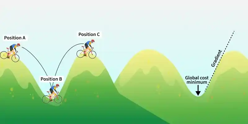
Imagine standing high up on a foggy mountain peak at night. Your goal is to reach the lowest valley floor (the point of minimum elevation), but you can only see a few feet in front of you.
  Elevation / Loss
        ▲
        │  *  (Starting Position - High Loss)
        │   \
        │    \  Steep Slope ──► Takes Larger Steps
        │     \
        │      \
        │       \  Gentler Slope ──► Takes Smaller Steps
        │        ╰─────────┐
        │                  ▼  (Valley Floor - Minimum Loss)
        └─────────────────────────────────────────────► Parameters (w)
How do you navigate down safely?
-
You feel the ground beneath your feet to determine which direction slopes downward most steeply.
-
You take a step in that downward direction.
-
You re-assess the slope at your new position and repeat the process step-by-step until the ground flattens out.
In machine learning:
-
The Mountain Elevation represents the Loss Function (or Cost Function), which measures how wrong your model’s predictions are.
-
The Valleys represent parameter values that minimize model error.
-
Your Step Direction and Size are calculated using Gradients and a scaling factor called the Learning Rate.
2. The Mathematics: Step-by-Step
A. The Loss Function $J(w)$
Let $J(w)$ represent our Loss Function, which depends on a parameter (weight) $w$. Our goal is to find the optimal weight $w^*$ where $J(w)$ reaches its global minimum.
B. The Gradient $\nabla J(w)$
The gradient is simply the derivative (slope) of the loss function with respect to the weight parameter:
$$\text{Gradient} = \frac{d J(w)}{d w}$$
-
If the slope is positive, the function is rising; to go downhill, move $w$ to the left (decrease $w$).
-
If the slope is negative, the function is falling; to go downhill, move $w$ to the right (increase $w$).
Because the gradient vector points in the direction of steepest ascent (uphill), we subtract the gradient to move in the direction of steepest descent (downhill).
C. The Parameter Update Rule
At each iteration $t$, update the weight parameter using the fundamental update equation:
$$w_{t+1} = w_t – \alpha \cdot \frac{d J(w_t)}{d w_t}$$
Where:
-
$w_t$ is the current weight parameter.
-
$\alpha$ (alpha) is the Learning Rate (a hyperparameter determining step size).
-
$\frac{d J(w_t)}{d w_t}$ is the derivative of the loss function evaluated at $w_t$.
3. The Crucial Role of the Learning Rate ($\alpha$)
The learning rate controls how aggressively the algorithm steps down the slope. Selecting the wrong learning rate leads to common optimization failures:
    Learning Rate Too Large                     Learning Rate Too Small
  (Overshoots & Diverges)                     (Painfully Slow Convergence)

        ▲   / \   /                             ▲  \
        │  /   \ /                              │   \ •
        │ /     X                               │    \ •
        │/     / \                              │     \ •
        └──────────►                            └──────────►
-
Too Small ($\alpha \ll 0.001$): Takes tiny incremental steps. Training is extremely slow and can get trapped in shallow local minima or flat plateaus.
-
Too Large ($\alpha \gg 0.1$): Overshoots the valley floor completely. The loss bounces wildly across the curve and may diverge toward infinity.
-
Just Right: Fast initial progress on steep slopes, naturally slowing down near the minimum to land smoothly at the optimal parameter value.
4. The Three Primary Variants of Gradient Descent
Depending on how much data is passed to calculate the gradient during a single update step, gradient descent is executed in three ways:
                           Gradient Descent Variants
                                       │
            ┌──────────────────────────┼──────────────────────────┐
            ▼                          ▼                          ▼
  [ Batch Gradient Descent ]  [ Stochastic (SGD) ]    [ Mini-Batch Gradient Descent ]
  • Uses ALL data per step    • Uses 1 random row    • Uses small batches (32-256)
  • Stable, but very slow      • Fast, but noisy     • Best of both worlds (Industry Standard)
| Variant | Data Used Per Update | Pros | Cons |
| Batch Gradient Descent | Entire dataset ($N$ rows) | Stable, smooth convergence curve | Computationally expensive; fails on massive datasets |
| Stochastic Gradient Descent (SGD) | $1$ random observation | Ultra-fast; escapes local minima easily | Extremely noisy updates; erratic convergence curve |
| Mini-Batch Gradient Descent | Small batches (e.g., $32, 64, 128$) | Fast GPU parallelization; stable convergence | Requires tuning batch size hyperparameter |
5. Advanced Optimizers Built on Gradient Descent
In modern deep learning frameworks, standard SGD is often upgraded with adaptive algorithms that automatically adjust step sizes:
-
Momentum: Adds a fraction of the previous update vector to the current step, building momentum to slide through flat regions and dampening oscillations.
-
RMSprop: Scales the learning rate inversely based on the moving average of recent squared gradients to balance updates across features.
-
Adam (Adaptive Moment Estimation): Combines the benefits of both Momentum and RMSprop. It maintains separate adaptive learning rates for every parameter and is the industry-standard default optimizer for neural networks.
Key Takeaway
Gradient descent calculates the direction of steepest slope (the derivative) and steps iteratively in the opposite direction to minimize model error. Mastering the interaction between the learning rate, loss function curve, and batching strategies is essential for training high-performing machine learning systems.